In the last blog I talked about the challenge to rural utilities, many of which serve relatively few people and have used federal monies to pay for a lot of their infrastructure.  In this blog we will take a look at the trends for community water systems which are defined as systems that serve at least 15 service connections or serve an average of at least 25 people for at least 60 days a year. EPA breaks the size of systems down as follows:

• Very Small water systems serve 25-500 people
• Small water systems serve 501-3,300 people
• Medium water systems serve 3,301-10,000 people
• Large water systems serve 10,001-100,000 people
• Very Large water systems serve 100,001+ people

Now let’s take a look at the breakdown (from NRC 1997).  In 1960, there were about 19,000 community water utilities in the US according to a National Research Council report published in 1997.  80% of the US population was served.  in 1963 there were approximately 16,700 water systems serving communities with populations of fewer than 10,000; by 1993 this number had more than tripled—to 54,200 such systems. Approximately 1,000 new small community water systems are formed each year (EPA, 1995). In 2007 there were over 52,000 community water systems according to EPA, and by 2010 the number was 54,000.  85% of the population is served. So the growth is in those small systems with incidental increases in the total number of people served (although the full numbers are more significant). 

TABLE 1 – U.S. Community Water Systems: Size Distribution and Population Served

Updating these numbers, there are over 54,000 systems in the US, and growth is almost exclusively in the very small sector.  93% are considered to be small or very small systems—serving fewer than 10,000 people. Even though these small systems are numerous, they serve only a small fraction of the population. Very small systems, those that serve 3,300 people or fewer make up 84 percent of systems, yet serve 10 percent of the population.  Most critical is the 30,000 new very small systems that serve only 5 million people (averaging 170 per system).  In contrast, the very large systems currently serve 45% of the population.  Large plus very large make it 80%.  The 800 largest systems (1.6%) serve more than 56 percent of the population. 900 new systems were added, but large systems served an additional 90 million people.

What this information suggests if that the large and very large sector has the ability to raise funds to deal with infrastructure needs (as they have historically), but that there may be a significant issue for smaller, rural system that have grown up with federal funds over the past 50 years.  As these system start to come to the end of their useful life, rural customers are in for a significant rate shock. Pipeline average $100 per foot to install.  In and urban area with say, 60 ft lots, that is $3000/household.  In rural communities, the residents may be far more spread out.  As an example, a system I am familiar with in the Carolinas, a two mile loop served 100 houses.  That is a $1.05 million pipeline for 100 hours or $10,500 per house.  With dwindling federal funds, rural customers, who are already making 20% less than their urban counterparts, and who are used to very low rates, that generally do not account for replacement funding, will find major sticker shock. 

This large number of relatively small utilities may not have the operating expertise, financial and technological capability or economies of scale to provide services or raise capital to upgrade or maintain their infrastructure.  Keep in mind that small systems have less resources and less available expertise.  In contrast the record of large and very large utilities, EPA reports that 3.5 percent of all U.S. community water systems violated Safe Drinking Water Act microbiological standards one or more times between October 1992 and January 1995, and 1.3 percent violated chemical standards, according to data from the U.S. Environmental Protection Agency (EPA).. 

EPA and professionals have long argued that centralized infrastructure for water and sewer utilities makes sense form an economy of scale perspective.  Centralized drinking water supply infrastructure in the United States consists dams, wells, treatment plants, reservoirs, tanks, pumps and 2 million miles of pipe and appurtenances.   In total this infrastructure asset value is in the multi-trillion dollar range.  Likewise centralized sanitation infrastructure in the U.S. consists of 1.2 million miles of sewers and 22 million manholes, along with pump stations, treatment plants and disposal solutions in 16,024 systems.  It is difficult to build small reservoirs, dams, and treatment plants as they each cast far more per gallon to construct than larger systems.  Likewise operations, despite the allowance to have less on-site supervision, is far less per thousand gallons for large utilities when compared to small ones.  The following data shows that the economy-of-scale argument is true:

• For water treatment, water distribution, sewer collection and wastewater treatment, the graphics clearly demonstrated the economy-of-scale of the larger utility operations versus small scale operations (see Figures 2-5). 
• The administrative costs as a percentage of the.total budget parameter also demonstrated the economy-of-scale argument that larger utilities can perform tasks at a lesser cost per unit than the smaller utilities (see Figure 6).

Having reviewed the operations costs, the next step was to review the existing rates.  Given the economy-of-scale apparent in Figures 2 to 6, it was expected that there would be a tendency for smaller system to have higher rates.  Figures 2-6 demonstrate this phenomena. 

So what to do?  This is the challenge.  Rate hikes are the first issue, a tough sell in areas generally opposed to increases in taxes, rates and charges and who use voting to impose their desires.  Consolidation is anothe5r answer, but this is on contrast to the independent nature of many rural communities.  Onslow County, NC  figured out this was the only way to serve people efficiently 10 years ago, but it is a rougher sell in many, more rural communities.  Infrastructure banks might help, the question is who will create them and will the small system be able to afford to access them.  Commercial financing will be difficult because there is simply not enough income to offset the risk.  The key is to start planning now for the coming issue and realize that water is more valuable than your iPhone, internet, and cable tv.  In most cases we pay more for each of them than water (see Figure 7).  There is something wrong with that…

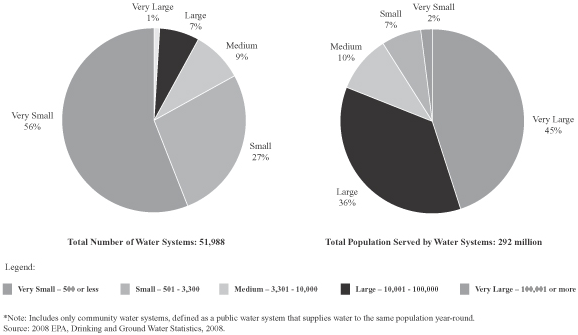
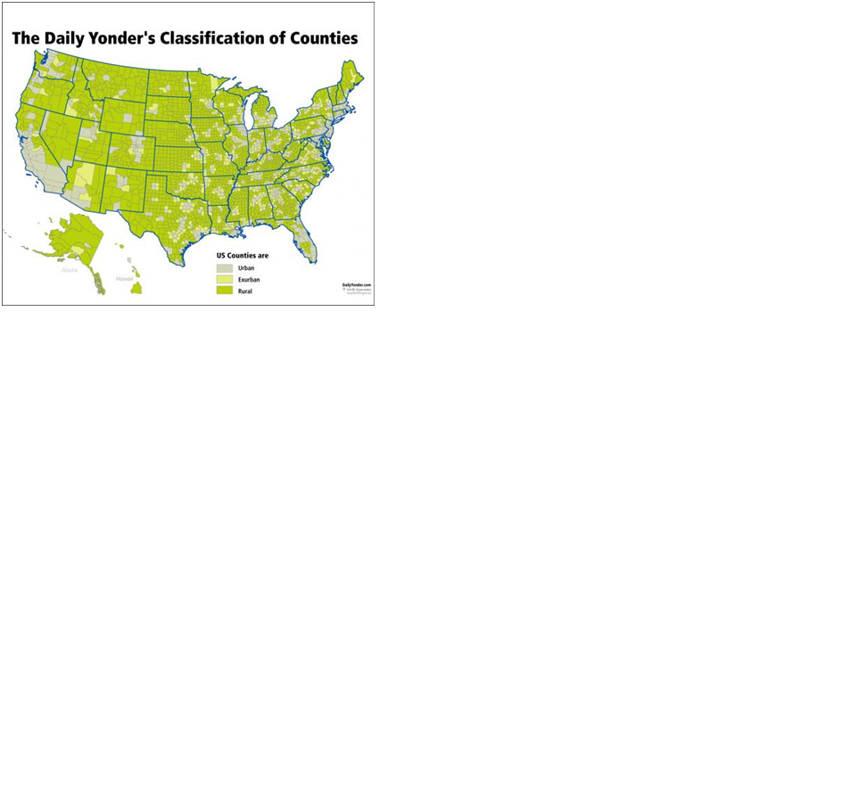
Figure 1  Breakdown of Size of Systems

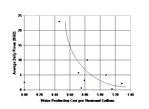
Fig 2 Cost of Water Treatment

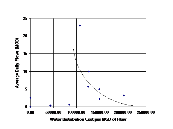
Fig 3 Cost of Water Distribution

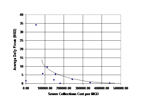
Fig 4 Cost of Sewer Collection

Fig 5 Cost of Sewer Treatment

Fig 6 Cost of Administration as a percent of total budget

FIgure 7 Water vs other utilities