A utility’s novel attempt to force farmers to curb pollution in rivers failed. Now the utility is on the hook for millions of dollars to protect the region’s drinking water.
— Read on www.governing.com/topics/transportation-infrastructure/gov-des-moines-water-utility-lawsuit-farmers.html
Tag Archives: sustainability
Transportation Lockboxes: The Road Funding Policy That Doesn’t Improve Roads Much
Voters in red and blue states like them. But historically, transportation “lockboxes” do little to address transportation problems.
— Read on www.governing.com/topics/transportation-infrastructure/gov-connecticut-transportation-lockbox-ballot-states.html
Controlling Algae?
The most important parameters regulating algal growth are nutrient quantity and quality, light, pH, turbulence, salinity and temperature. Light is the most limiting factor for algal growth, followed by nitrogen and phosphorus limitations, but other nutrients are required including carbon. Biomass is usually measured by the amount of chlorophyll a in the water column. Water temperature influences the metabolic and reproductive rates of algae. Most species grow best at a salinity that is slightly lower than that of their native habitat, The pH range for most cultured algal species is between 7 and 9, with the optimum range being 8.2-8.7. Through photosynthesis, algae produce oxygen in excess of respiratory requirements during daylight hours. Conversely, during low light or nighttime periods algae respire (consume) dissolved oxygen, sometimes depleting water column concentrations. Thus, high algae concentrations may lead to low dissolved oxygen concentrations.
A common solution for algae is copper sulfate. Copper Sulfate works to kill the algae, but when it dies, it settles to the bottom of the water body where it becomes a carbon source for bacteria and future algae. One will often see shallow ponds with rising algae. But there is significant concern about copper in coastal water bodies. Copper is toxic to marine organisms so USEPA and other regulatory bodies are considering the limits on copper use. Such a limitation would severely limit options in dealing with algal blooms near coastal waters.
Mixing is necessary to prevent sedimentation of the algae, to ensure that all cells of the population are equally exposed to the light and nutrients. So oxygenation can help (it also mixes the water. The depth of south Florida water bodies is problematic (shallow and therefore warmer than normal). But oxygen will help microorganisms on the bottom consume the carbon source on the bottom, which might slow algal growth. Analysis is ongoing.
Two other conditions work against controlling blue-green algae outbreaks: climate change and political/regulatory decision-making. Lake Okeechobee has routine algal blooms from the nutrients introduced from agriculture and runoff around the lake, which encouraged an artificial eutrophication of the lake years ago. It continues today. Warmer weather will encourage the algal blooms in the future. The decisions to discharge the water without treatment is a political one. From a regulatory perspective, algae is seen as a nuisance issue, not a public health or environmental issue. But algal blooms consume oxygen and kill fish, so the ecosystem impact is considerable – it is not a nuisance .
Algae Part 2 – So what is this stuff?
The term algae encompass a variety of simple structures, from single-celled phytoplankton floating in the water, to large seaweeds. Algae can be single-celled, filamentous or plant-like, anchored to the bottom. Algae are aquatic, plant-like organisms – phytoplankton. Phytoplankton provides the basis for the whole marine food chain. Phytoplankton need light to photosynthesize so will therefore float near the top of the water, where sunlight reaches it. Light is the most limiting factor for algal growth, followed by nitrogen and phosphorus limitations), but other nutrients are required including carbon, silica, and other micronutrients. These microscopic organisms are common in coastal areas. They proliferate through cell division.
A natural progression occurs in many water bodies, from diatoms, to green algae to yellow/brown to blue-green, with time and temperature. The environment is important. Southern waters are characterized as being slow moving, and warm. This encourages cyanobacteria – or blue green algae. The introduction of nutrients is particularly difficult as it accelerates the formation of the blue green algae. Blue-green algae creates the bright green color, but is actually an end-of-progression organism.
If cells are present in the water mass in large numbers an algal bloom occurs. An algal bloom is simply a rapid increase in the population of algae in an aquatic system. Blooms may occur in freshwater as well as marine environments. Colors observed are green, bright green, brown, yellowish-brown, or red, although typically only one or a few phytoplankton species are involved and some blooms may be recognized by discoloration of the water resulting from the high density of pigmented cells.
So the desire for development created the idea to drain the swamp, which led to exposure of dark, productive soil that led to farming, which lead to fertilizers, which led to too much water, and water pollution leading to algae. A nice, predictable progression created by people. So what is the solution?
Algae Algae everywhere – Where’s a Fish to think?
We have all seen the stories about land in the Everglades agricultural Area thissummer. I was asked to give a presentation at a national conference in Orlando recently about water management in Florida. It was a fun paper and most of the people there were not from Florida, so it was useful for them to understand the land of water. Florida has always been a land shaped by water. Initially it was too much, which frustrated federal soldiers trying to hunt down Native Americans in the 1830s. In 1881, real estate developer Hamilton Disston first tried to drain the swamps with canals. He was not successful, but Henry Flagler came through a decade later and constructed the east coast railroad in the 1890s. It is still there, 2 miles off the coast, on the high ground. However water limited development so in 1904, Napoleon Bonaparte Broward campaigned to drain the everglades. Broward’s efforts initiated the first land boom in Florida, although it was interrupted in the 1920s by hurricanes (1926 and 1928) that sloshed water out of Lake Okeechobee killing people and severely damaging property in Miami and around Lake Okeechobee. A dike was built (the Hover dike – it is still there). However, an extended drought occurred in the 1930s. With the dike preventing water from leaving Lake Okeechobee, the Everglades became parched. Peat turned to dust, and saltwater entered Miami’s wells. When the city brought in an expert to investigate, he found that the water in the Everglades was the recharge area for the Biscayne aquifer, the City’s water supply. Hence water from the lake needed to move south.
Resiliency has always been one of Florida’s best attributes. So while the hurricanes created a lot of damage, it was only a decade or two later before the boom returned. But in the late 1940s, additional hurricanes hit Florida, causing damage and flooding from Lake Okeechobee prompting Congress to direct the Army Corps of Engineers to build 1800 miles of canals, dozens of pump stations and other structures to drain the area south of Lake Okeechobee. It is truly one of the great wonders of the world – they drained half a state by lowering the groundwater table by gravity canals. To improve resiliency, between 1952 and 1954, the Corps, in cooperation with the state of Florida, built a levee 100 miles long between the eastern Everglades and the developing coastal area of southeast Florida to prevent the swamp from impacting the area primed for development.
As a part of the canal construction after 1940, 470,000 acres of the Everglades was set aside for farming on the south side of Lake Okeechobee and designated as the Everglades Agricultural Area (EAA). However water is inconsistent, so there are ongoing flood/drought cycles in agriculture. Irrigation in the EAA is fed by a series of canals that are connected to larger ones through which water is pumped in or out depending on the needs of the sugar cane and vegetables, the predominant crops. Hence water is pumped out of the EAA, laden with nutrients. Backpumping to Lake Okeechobee and pumping the water conservation areas was a practice used to address the flooding problem.
There was an initial benefit to Lake Okeechobee receiving nutrients. Older folks will recall that in the 1980s , the lake was the prime place for catching lunker bass. That was because the lake was traditionally nutrient poor. That changed with the backpumping which stimulated the biosystem productivity. More production led to more biota and more large fish. This works as long as the system is in balance e- i.e. the nutrients need to be growth limiting at the lower end of the food chain. Otherwise the runaway nutrients overwhelm the natural production and eutrophication results. Lake Okeechobee is a runaway system – the algae now overwhelm the rest of the biota. Lunker bass have been gone for 20 years.
The backpumped water is usually low in oxygen and high in phosphorus and nitrogen, which triggers algal progressions, leading to toxic blue-green algae blooms and threaten lake drinking water supplies. Think Toledo. Prolonged back pumping can lead to dead zones in the lake, which currently exist. The nutrient cycle and algal growth is predictable.
The Hoover Dike is nearly 100 years old and while it sit on top of the land (19 ft according to the Army Corps of Engineers), there is concern about it being breached by sloshing or washouts. Undermining appears in places where the water moves out of the lake flooding nearby property. So the Corps tries to keep the water level below 15.5 ft. During the rainy season, or a rainy winter as in 2016, that can become difficult. If the lake is full, that nutrient laden water needs to go somewhere. The only options are the Caloosahatchee, St. Lucie River or the everglades. The Everglades is not the answer for untreated water – the upper Everglades has thousands of acres of cattails to testify to the problem with discharges to the Everglades. So the water gets discharged east and west via the Caloosahatchee and St. Lucie River.
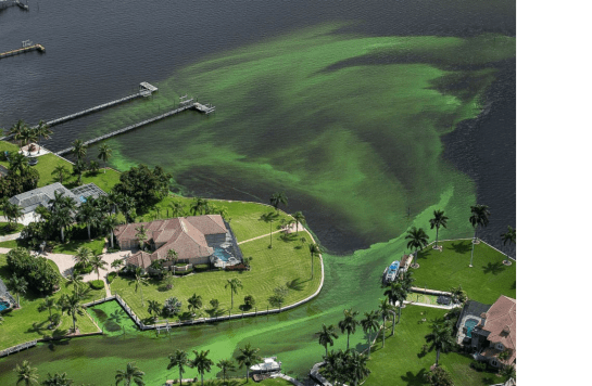
The nutrient and algae laden water manifests as a green slime that washed onto Florida beaches in the Treasure coast and southwest Florida this summer, algae is actually a regular visitor to the coasts. Unfortunately memories often fail in temporal situations. The summer 2016 occurrence is reportedly the eighth since 2004, and the most severe since 2013. The green slime looks bad, can smell bad, kills fish and the 2016 bloom was so large it spread through estuaries on both coasts killing at least one manatee. One can see if from the air – try this link:
The Costs of SLR and Rainfall
The reliability of the assets within the area of interest starts with the design process in the asset management plan. Decision-making dictates how the assets will be maintained and effective means to assure the maximum return on investments. Through condition assessment, the probability of failure can be estimated. Assets can also fail due to a growing area that may contribute to exceeding its maximum capacity. Operation and maintenance of the assets are important in reassuring a longer life span as well as getting the most out of the money to be spent. Prioritizing the assets by a defined system will allow for the community to see what areas are most susceptible to vulnerability/failure, which assets need the most attention due to their condition, and where the critical assets are located in relation to major public areas (hospitals, schools, etc.) with a high population.
So what happens when conditions change? Let’s say sea levels are rising and your land is low. What would the potential costs be to address this? Better yet, what happens if it rains? We looked at one south Florida community and the flood stage for each based on 3 storm events: the 1:10 used by FDOT (Assumes 2.75 inches in 24 hours), the Florida Building Code event that includes a 5 in in one hour event (7 in in 24 hrs), and the 3 day 25 year event (9.5-11 inches).
Of no surprise is that the flooding increases as rainfall increases. Subsequent runs assumed revisions based on sea level rise. The current condition, 1, 2 and 3 ft sea level rise scenarios were run at the 99 percentile groundwater and tidal dates and levels. Tables 2-5 depict the flood stage results for each scenarios. The final task was designed to involve the development of scenarios whereby a toolbox options are utilized to address flooding in the community. Scenarios were to be developed to identify vulnerabilities and cost effectiveness as discussed previously.
The modeling results were then evaluated based of the accompanying infrastructure that is typically associated with same. A summary of the timelines and expected risk reductions were noted in the tables associated with storm and SLR scenarios. This task was to create the costs for the recommended improvements and a schedule for upgrading infrastructure will be developed in conjunction with staff. Two issues arise. First, the community needs to define which event they are planning to address and the timelines as the costs vary form an initial need of $30 million to over $300 million long-term. Figure 1 shows how these costs rise with respect to time. The long-term needs of $5 million per 100 acres matches with a prior effort in Palm Beach County.
Figure 1 Summary of Costs over the 3 ft of potential sea level Rise by 2011, under the 3 storm planning concepts.
4% Doesn’t Sound Like Much….
The average is 4% of visible infrastructure is in poor condition. Actually 4-6% depending on the municipality. And this was visible infrastructure, not buried, but there is not particular reason to believe the below ground infrastructure is somehow far worse off. Or better. That 4-6% is infrastructure that needs to be fixed immediately, which means that as system deteriorate, there is catch –up to do. The good news is many of the visible problems were broken meter boxes, damaged valve boxes, broken curbs and broken cleanouts- minor appearing issues, but ones that likely require more ongoing maintenance that a water main. And the appearance may be somewhat symptomatic – people perceive that the system is rundown, unreliable or poorly maintained when they see these problems. It raises a “Tipping Point” type discussion. “Tipping Points” Is a book written by Malcolm Gladwell that I read last year (great book – my wife found it in a book exchange for free in Estes Park last summer). It was along a similar vein of thought as the Freakanomics books – the consequences of certain situations may be less clear than one thinks. The Tipping point that is most relevant is crime in New York in the early 1990s after Bernard Goetz shot several assailants in the subway. The problem was significant and the subways were thought to be among the higher risk areas. The new police chief and Mayor decided that rather that ignore the petty crimes (like many large cities do), they would pursue those vigorously. So fare hopping on the train and the like were challenged immediately. They decided that no graffiti would be visible on the subways and cleaned cars every night to insure this remained the case. Cars with graffiti were immediately removed from service. New subway cars were ordered. Pride and public confidence improved. Crime dropped. The impact of their efforts was that people recognized that criminal behavior would not be tolerated and fairly quickly criminal activity decreased. It was a big success story, but the underlying reasons were less discussed, but easily transferrable to our infrastructure. If we have broken valve boxes, meters, cleanouts, storm drains etc., the same perceptions of a rundown community rise. Rundown communities lead to a loss of public confidence and trust and pride. And none of those help our mission or our efforts to increase infrastructure spending. 4% might not look like much, but it can drastically change the perception of the community. So let’s start to fix those easy things; and document that we did in our asset management programs.
Forest Fires
My grandmother lost here summer cabin outside of Grayling, Michigan in the Great Crawford County fire on 1990. My grandfather had hauled the cabin and out buildings up to Grayling by rail from Detroit in the 1920s (some old houses my Great Grandmother had owned). It was one of many fires that year, but an early one caused by significantly less snow over the prior winter, high winds, and carelessness. The cabin was gone before anyone could react as it appears to have been in the dead center of the moving flames. I recall the story on CNN, but no one realized exactly where it was. My grandmother never recovered. She wasn’t the only one. 20 year later there are trees.
Forest fires happen with increasing frequency. Today in Southern California, the Sand Fire has set more than 35,000 acres of the Santa Clarita Valley ablaze. Difficulties fighting it are not limited to temperatures hitting 101 degrees in the area and dried brush from 5 years of drought conditions. The Soberanes Fire in Monterey County has burned 16,100 acres along the California coast between Carmel and Big Sur. The fire is bigger than the size of Manhattan. The 778 acre McHugh Fire located on the steep terrain south of Anchorage, Alaska. Looking at the map, it seems the west is on fire. A larger and larger portion of the US Forest Services’ budget gets spent on fire-fighting each year – 67% in 2016. Yet fires on Forest Service property account for only 20% of the total fire nationally (1.9 million acres or a total of over 10 million acres in 2015), but this total amount is increasing. Warmer weather in the west has increased the length of fire season, drought has increased the risk, budgets are stagnant so means to prevent fire intensity have been reduced, The only good news is that a University of Vermont study suggests that areas where pine beetle has killed trees is actually thinner and less at risk that heathier forests, if that is a “good” thing.
My friend Dr. Chi Ho Sham did some work on forest fires on watersheds a few year back. He found that forest fires have obvious impacts on people and our customers, but also our water supplies and our water supplies. The ash runs off into streams and is difficult to remove at water plants because it is so fine. Areas burned are far more subject to erosion after rain of snow melt thereby creating a need for more treatment at water plants. This will go on for some time after the rain until groundcover can re-establish itself. Fire retardant and water drops combat some fires although the retardant shows up in streams and water supplies with adverse impacts. Dams and reservoirs will need more frequent dredging due to buildup, and wildlife equilibrium will be disrupted. Forest fires make for interesting news, when they are far away, but few utilities think too much about what would happen if their watershed were impacts. No groundwater utility has thought about impacts on surficial groundwater although that might be an interesting study. But we should all have plans, should watch our watershed, and be cognizant that far away fires might give us the opportunity to study what could possibly go wrong at our utilities. Meanwhile, our thoughts are with those in the realm of the conflagrations. Be Safe!!
Current Fire map – July 2016 Sources; http://activefiremaps.fs.fed.us/
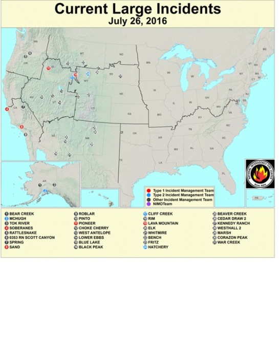
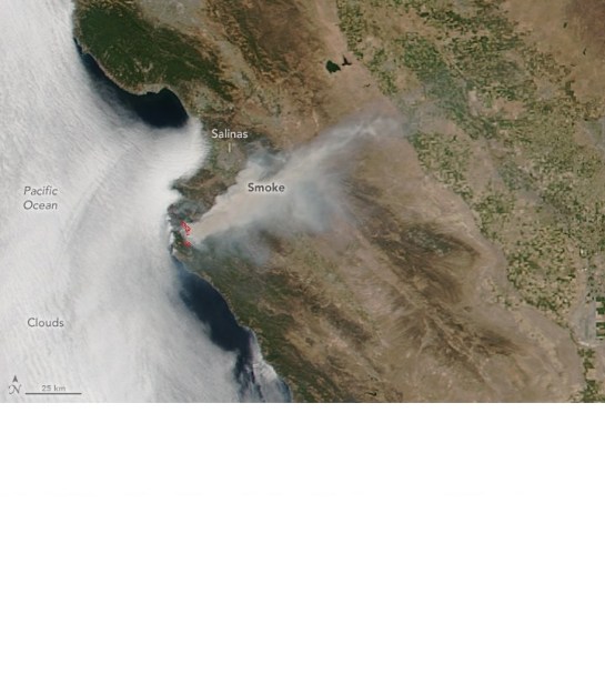
Satellite photo of fire outside San Francisco Source NASA Earth
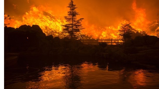
FIre outside Santa Clarita CA July 2016Source CNN
Alaska FIres
Oasis in Dania Beach with Student Help
Collaboration between students, faculty and the real world is an excellent means to integrate students into real world situation and provide them valuable experience. I have done this with several communities to date. Below are the installed OASIS street improvements in Dania Beach. Students did the drafting. Also a stormwater pipe in Boynton Beach. Excellent learning experience. The campus mapping project is one that our Facilities Management Department needed. Very cool 3D map. We did stormwater assessments in Davie, plus flood mapping. Of course the Dania Beach nanofiltration plant, the first LEED Gold water plant in the world. Still. Here is the cool thing with working with students – they have all kinds of ideas and have all kinds of tools that they can access – they just need guidance. They will create tools (our app for asset management). to make the job easier. Most collaborate well. And most want to learn about the profession. As an industry we should promote this more. Go to the local universities, talk with faculty. Find the right faculty mentor who is interested in local outreach. Work with them. But students should not work free. Pay or pay in grades. It’s only fair.
Asset Management and Condition Index
Here is an example of getting to a condition assessment with limited data using power point slides. Note that where there are categorical variables (type of pipe for example), these need to be converted to separate yes/no questions as mixing. Categorical and numerical variable do not provide appropriate comparisons = hence the need to alter. Take a look – but the concept is to predict how well this model explains the break history on this distribution system. Call me and we can try it on yours….
Step 1 Create a table of assets (this is a small piece of a much larger table).
Asset | Dia |
water main | 2 |
water main | 2 |
water main | 2 |
water main | 2 |
water main | 4 |
water main | 6 |
water main | 6 |
water main | 6 |
water main | 6 |
Step 2 Create columns for the variables for which you have data (age, material, soil type, groundwater level, depth, traffic, trees, etc.)
Asset | breaks in 10 year | Dia | Age | soil | traffic | Trees | depth | pressure | material | Filed estimate of cond.ition |
water main | 17 | 2 | 45 | 1 | 1 | 2 | 1 | 55 | 4 | 3 |
water main | 11 | 2 | 45 | 2 | 1 | 2 | 1 | 55 | 4 | 3 |
water main | 12 | 2 | 45 | 1 | 1 | 2 | 1 | 55 | 4 | 3 |
water main | 10 | 2 | 45 | 1 | 1 | 2 | 1 | 55 | 4 | 3 |
water main | 2 | 4 | 50 | 1 | 1 | 2 | 1 | 55 | 1 | 2 |
water main | 3 | 6 | 60 | 2 | 2 | 2 | 1 | 55 | 1 | 2 |
water main | 1 | 6 | 60 | 2 | 2 | 2 | 1 | 55 | 1 | 2 |
water main | 0 | 6 | 20 | 1 | 1 | 2 | 1 | 55 | 3 | 1 |
Step 3 All variables should be numeric. So descriptive variables like pipe material need to be converted to binary form – i.e. create a column for each material and insert a 1 or 0 for “yes” and “no.”
Step 4 Run Linear regression to determine factors associated with each and the amount of influence that each exerts. The result will give you a series of coefficients:
Step 5 – Use this to predict where your breaks will likely be in the next 5-10 years.
The process is time consuming but provides useful information on the system. It needs to be kept up as things change, but exact data is not really needed. And none of this requires destructive testing. Not bad for having no information.